
Kriging Concepts
Note
Coming in Spatial Integration version 3.
This page explains the ideas behind the Interpolation dialog. There is no mathematics in it. If you have used kriging before, skip ahead to How SI Differs from Conventional Kriging near the bottom - some of the choices here differ from a conventional mining package, and it is worth knowing which.
The Problem
You have drill holes. Between them you have nothing, and yet you need a value everywhere: a grade at every block, a density at every node, a geochemical value through the whole volume. Every method of filling that gap is a way of answering one question - when I estimate a point, how much should each nearby sample count?
The simplest answer is to weight samples by one over their distance, or the square of it. That is inverse distance weighting, and it is not unreasonable, but the weights are a guess. They take no account of how far your particular deposit stays continuous, of the fact that your mineralisation runs along strike rather than across it, or of the fact that three holes clustered together on one side of a block are, between them, telling you roughly one thing rather than three.
Kriging answers the same question by measuring rather than guessing. It first asks the data how quickly it changes with distance and direction, and then derives weights from that measurement. Everything on the Variogram tab exists to make that measurement.
Measuring Continuity: The Variogram
Take every pair of samples in your dataset. For each pair, note two things: how far apart they are, and how different their values are. Now group the pairs by separation - all the pairs about 25 m apart, all the pairs about 50 m apart, and so on - and for each group work out the average difference.
Plot those group averages against separation and you have an experimental variogram. Almost always it rises: samples close together are alike, samples far apart are not. What matters is how it rises, and where it flattens off.
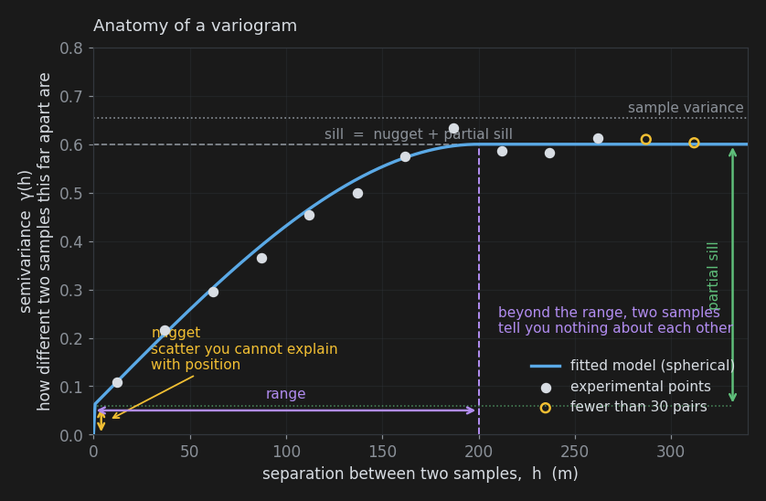
The vertical axis is semivariance, written γ(h). Treat it as "how different two samples this far apart tend to be" - it does not matter for practical work that it is half the average squared difference.
Three numbers describe the curve, and they are the three you will spend your time on.
Nugget
The height at which the curve starts, rather than at zero. If two samples taken from almost the same place still differ, that difference cannot be explained by their positions. It comes from sampling and assaying error, and from real variability at a scale finer than your sample length - the original gold-nugget effect that gives it its name.
The nugget is the honesty control of the whole estimate. A high nugget tells kriging that individual samples are unreliable, so it spreads weight widely and produces a smooth result that does not pass exactly through the sample values. A zero nugget tells kriging every sample is exact, and the estimate is forced through every one of them, warts and all.
Because the nugget lives at zero separation, you can only see it if you have pairs of samples very close together. Between holes, your closest pairs are a whole hole spacing apart, which is far too coarse. Only pairs within the same hole are close enough - which is why the workflow starts with a downhole variogram.
Range
The separation at which the curve flattens out. Beyond the range, two samples are no more alike than two chosen at random from anywhere in the deposit: they have nothing to say about each other. Inside the range, the closer they are, the more they have to say.
The range is the honest statement of how far your data reaches. If it comes back at 60 m and your holes are 120 m apart, you have not drilled your deposit closely enough to interpolate it - and the estimate will drift to the average in the middle of every gap, which is the correct answer given the data, if not the one anyone wanted.
Sill and Partial Sill
The height at which the curve flattens is the sill. Since the curve levels off at the point where samples are unrelated, the sill should land near the overall variance of your samples, which is drawn on the plot as a reference line. The partial sill is the part of that height above the nugget - the portion of the variability that position actually explains. The dialog asks for the nugget and the partial sill separately, because that is the split that matters: nugget is noise, partial sill is structure.
Model Shapes
The experimental points are noisy and only exist at the separations your drilling happens to provide. Kriging needs a smooth curve defined at every distance, so a model is fitted through the points. Three shapes are offered.
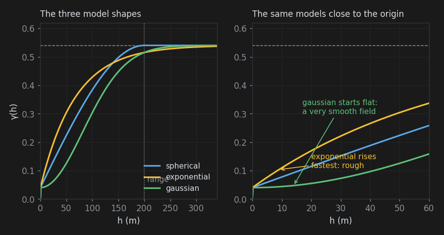
- Spherical reaches the sill exactly at the range and stays there. It is the workhorse of mining geostatistics and the right default.
- Exponential approaches the sill without ever quite reaching it, and rises more steeply near the origin. It suits noisier, less obviously bounded phenomena.
- Gaussian starts out flat before rising, which describes a very smooth, continuous field - a good fit for a thickness or an elevation, rarely for a grade. It is also numerically delicate: a Gaussian model with a nugget of zero will usually fail to solve.
The right-hand panel of the figure shows where the choice really bites. The first few metres of the curve - its shape near the origin - control the weight given to the closest samples, which dominates every estimate. Two models can score similarly overall and behave completely differently there, which is why the fit panel reports the short-lag error separately and warns you when the model badly overshoots the first experimental point.
Direction: Anisotropy
So far the variogram has been treated as if only distance mattered. In geology it rarely does. A stratabound horizon is continuous for hundreds of metres along strike and tens of metres across it; a plunging shoot is continuous down plunge and nowhere else. Continuity that depends on direction is called anisotropy, and describing it usually improves an estimate more than any other single change.
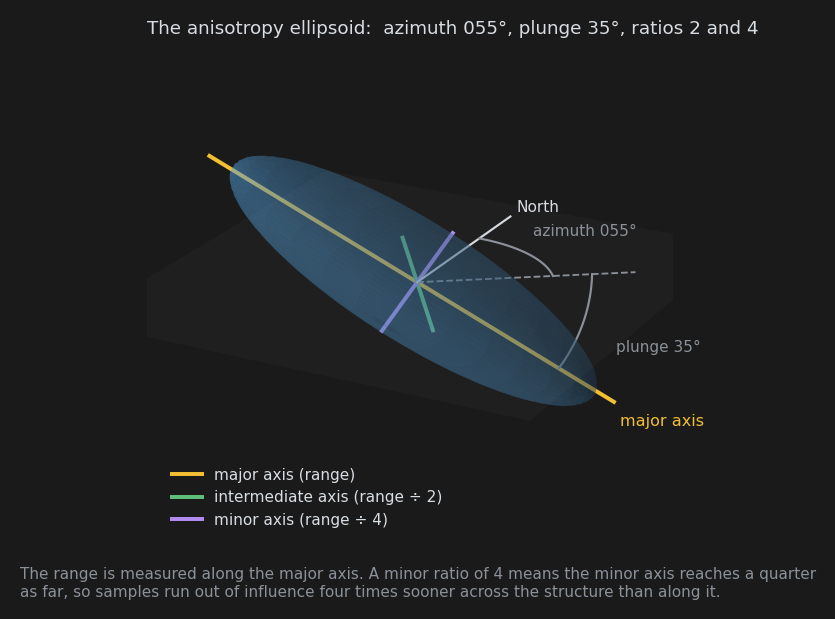
It is described as an ellipsoid: an orientation for the direction of best continuity, and two ratios saying how much shorter the other two directions are. The dialog can measure it for you. See Anisotropy for the full picture.
What Kriging Then Does
With a variogram model in hand, kriging works out the weights for each estimate so that the expected error is as small as it can be, given what the variogram says about the deposit. Three consequences are worth knowing about.
It declusters automatically. Three samples close together carry little more information than one, and the weights reflect that - the cluster shares out weight that a single isolated sample would keep for itself. No manual declustering is needed.
It respects direction. With anisotropy, a sample 200 m away along strike can carry more weight than one 80 m away across it. That is the whole point.
It smooths. Every estimate is an average of samples, and averages have less variability than the things they average. The grid will always be smoother than reality - it will show fewer very high and very low values than the ground contains.
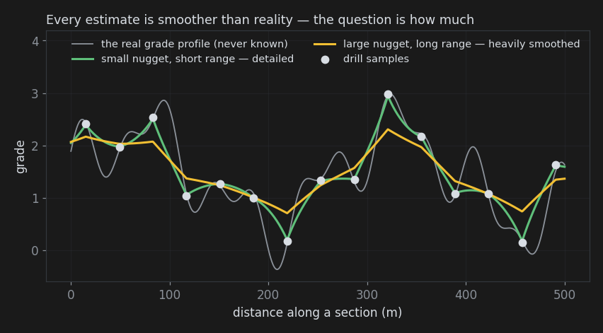
Smoothing is not a bug, but the amount matters. Too much and your high-grade zones dissolve into their surroundings, which shows up as a low regression slope on the Quality tab. The nugget, the range and the anisotropy ratios all control how much you get.
A related warning: the grid is a set of estimates, not a resource statement. Applying a cut-off to smoothed node values does not give a tonnage you can bank, because the smoothing has moved values across the cut-off in both directions. Use the grid to understand and communicate shape, continuity and trend.
How SI Differs from Conventional Kriging
For readers who know kriging from other software, these are the things worth knowing.
- The estimate is solved for all samples at once. The covariance model, anisotropy and drift are the ones you would recognise, and for a given variogram the estimates are kriging estimates. Rather than setting up a small system of equations at each node, SI solves once for the whole dataset and then evaluates the result at every node.
- There is no search neighbourhood. No minimum or maximum sample count, no search radius, no octant search. Every sample contributes to every node; the variogram range is what makes distant samples irrelevant. This removes a family of artefacts caused by the sample set changing abruptly from node to node, and it removes a family of controls you may be used to reaching for.
- Estimates are at points, not blocks. Each grid node carries an estimate for that point. There is no block discretisation or change of support.
- Ordinary kriging by default, with an optional linear drift. Ordinary kriging assumes the mean is constant but unknown locally, which is the usual choice. The linear drift option (universal kriging) suits data with a genuine regional trend, and will extrapolate that trend beyond your data - vigorously.
- There is no kriging variance. Solving for all samples at once does not produce one, and nothing else is offered in its place. Instead, every grid carries a distance to nearest sample array, which is a statement about data coverage rather than uncertainty, and the Quality tab provides cross validation, which is an honest measurement of error rather than a model-derived one.
- Values are used as they are. No transform, top-cut or declustering is applied to the values before estimation. If your data is strongly skewed, or mixes populations, deal with it by restricting the run to one domain rather than expecting the estimator to sort it out.
Vocabulary
| Term | Meaning |
|---|---|
| Lag | A distance band that sample pairs are grouped into, e.g. all pairs 25 m apart give or take 12.5 m |
| Semivariance, γ(h) | How different two samples separated by distance h tend to be |
| Nugget | Variability at zero separation: sampling error plus structure finer than your samples |
| Sill | The height the variogram flattens off at, near the sample variance |
| Partial sill | Sill minus nugget: the variability that position explains |
| Range | Separation beyond which samples are unrelated |
| Anisotropy | Continuity that depends on direction |
| Drift | A regional trend in the mean, rather than a constant mean |
| Kernel | The covariance model used for the estimate; each variogram model shape has a matching kernel |
| Cross validation | Hiding some samples, estimating them from the rest, and comparing |
Also See
- Interpolation - the workflow overview
- Variogram tab - measuring all this from your own data
- Quality tab - checking the result