Volumes – Spatial Integration

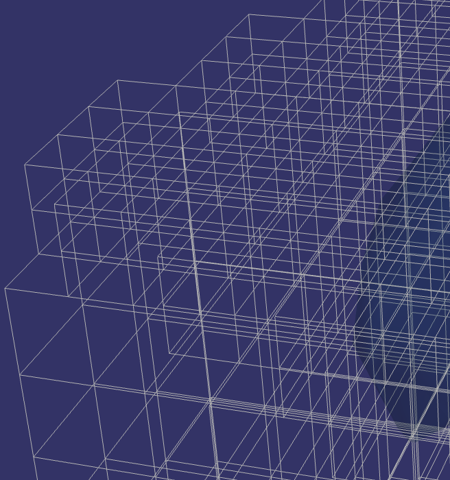
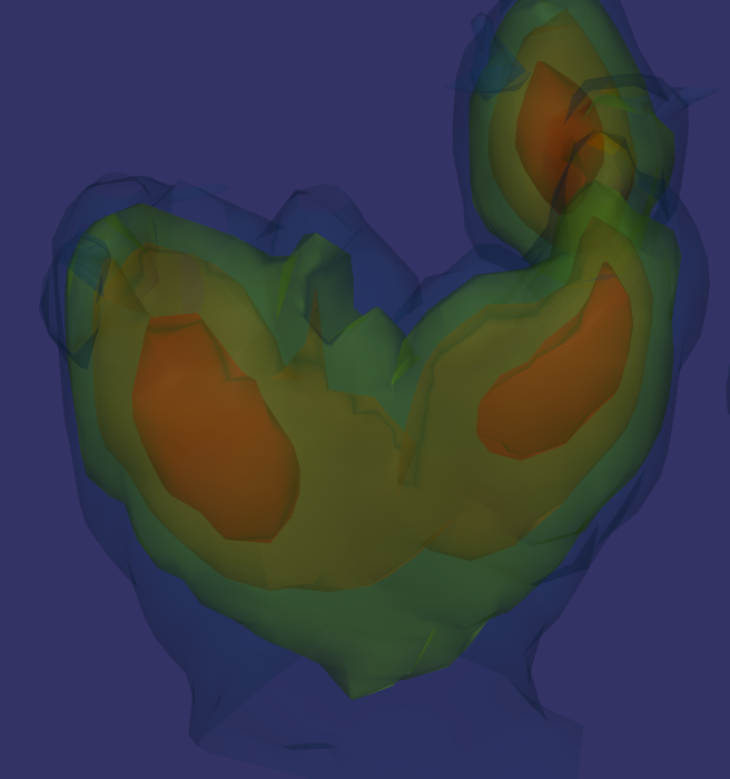
Volumes discretise any 3D space into cells or blocks, with one or more attributes per cell or per corner. Typical volumes are block models of ore grades and 3D geophysics inversions of magnetics, gravity etc.

Volumes can be descretised in many ways. Spatial Integration covers them all:

Image – All cells are the same size. This produces a regular grid.
Rectilinear – Rows, columns and levels of the grid can change size, but all cells in that row, column or level have the same size. This produces a regular grid of varying size cells. Also known as Tensor meshes.
Structured – A regular grid with every cell joining its neighbours at the corners, but the cells can be trapezoidal to form curved grids.
Unstructured – Each cell does its own thing. Every grid can be represented as an unstructured grid, but it takes longer to process due to the irregular topology. Non-rectangular cells (eg tetrahedral meshes) can also be represented this way.
Tree – The entire grid volume is covered by 1 (or a small number) of root cells. These subdivide into smaller cells in areas that require more detail, then those cells subdivide again if still more detail is required. Usually a cell will subdivide into 8 subcells, 2 in each direction. These grids are great for covering a large space at varying resolutions. Examples are VTK HyperTree grids and UBC Octree meshes.

Supported Formats

`Format`	`Description`
.vti	VTK Image Data (XML) – regular image grid
.vts	VTK Structured Grid (XML) – curvilinear structured grid
.vtr	VTK Rectilinear Grid (XML) – tensor/rectilinear grid
.vtu	VTK Unstructured Grid (XML) – arbitrary cell topology
.vth	VTK HyperTree Grid (XML) – adaptive tree grid
.vtk	VTK Legacy format – any of the above grid types
.mesh, .msh	Discretise / SimPEG Tensor Mesh – requires a separate model file containing attribute values
.mesh, .msh	Discretise / SimPEG Tree Mesh (OcTree) – requires a separate model file containing attribute values
.dcm, .dicom	DICOM medical image – can load a single file or all files in a directory. You can also select a DICOM index file
.xyz	Loke XYZ IP/Resistivity inversion output
.dat	Micromine block model (Extended Data File) – supports rotated and sub-blocked models. Text fields are loaded as numeric category indices

Note: If you have a legacy .vtk file or another slow-to-load format (eg UBC Tensor/Tree mesh), Spatial Integration can convert it to the equivalent modern XML format for you before loading. Tick the Convert to modern VTK prior to loading option in the Volume Settings dialog. The converted file is saved alongside the original and will be used automatically next time.

Loading a Volume

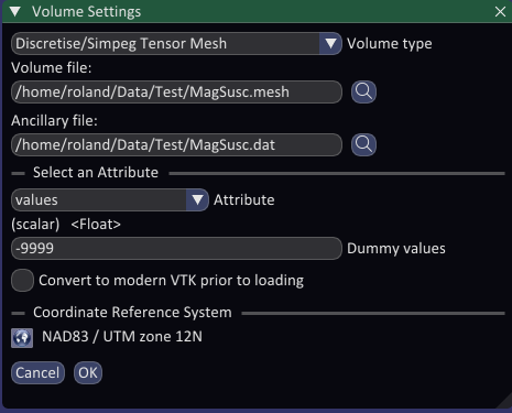
Select Add Volume from the volume flyout menu to open the Volume Settings dialog.

Volume type – This will normally be determined from the volume file once you choose one. You only need to manually select the volume type if the automatic selection hasn’t been able to figure out the type.
Volume file – Click the browse button to locate your volume file. After selecting a file, Spatial Integration will attempt to read the available attributes and populate the attribute selector. For DICOM data you can tick Use all files in directory to load a full image stack from a folder rather than a single slice.
Ancillary file – If the volume type requires another file with attribute data (eg UBC Simpeg/Discretise formats), a second file browse field will appear.
Attribute – Choose the data column or array you want to load from the list. Only numeric attributes are shown. A brief summary of the selected attribute (type and size) is displayed below the selector.
Dummy values – If your data uses one or more special values to indicate missing or invalid cells (sometimes called null or no-data values), enter them here separated by spaces. Cells matching these values will be hidden from all visualisations. Nan (not-a-number) values are automatically used as dummy values and don’t need to be listed in the text box.
Convert to modern VTK – Available for non-modern VTK formats, including legacy .vtk files. Tick this to convert the file to the modern XML format before loading. The converted file is saved next to the source file with the same name.
Coordinate Reference System – Click the CRS button to assign a projected coordinate system to the volume. If the file embeds a CRS or there is a qpj file with the same filename it will be detected and displayed automatically. Without a CRS, the view CRS is assumed and you can only display the volume in Projected coordinate systems.

Click OK to load the volume. It will appear in the scene and in the layer list, ready to be visualised.

Visualisations

Once a volume is loaded, Spatial Integration provides several visualisation types. Each can be added via the layer context menu and configured from the symbology panel. Isosurface and Outline visualisation are added by default, although the Outline is not visible by default.

Isosurface

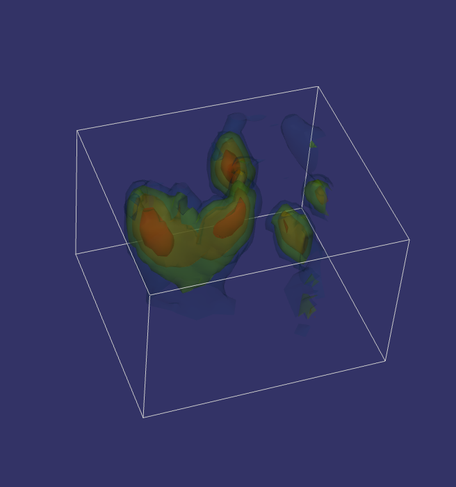
An isosurface is a 3D triangulated surface drawn at the boundary where the attribute equals a chosen value. It is the 3D equivalent of a contour line on a map. Isosurfaces are the primary way to visualise the shape and extent of features within a volume, for example an ore grade shell or a conductivity anomaly.

You can add multiple isosurfaces to a single layer, each with its own isovalue, colour and opacity. When the isovalue slider is dragged a fast preview is shown using a downsampled grid; releasing the slider or entering a value triggers the full-resolution calculation.

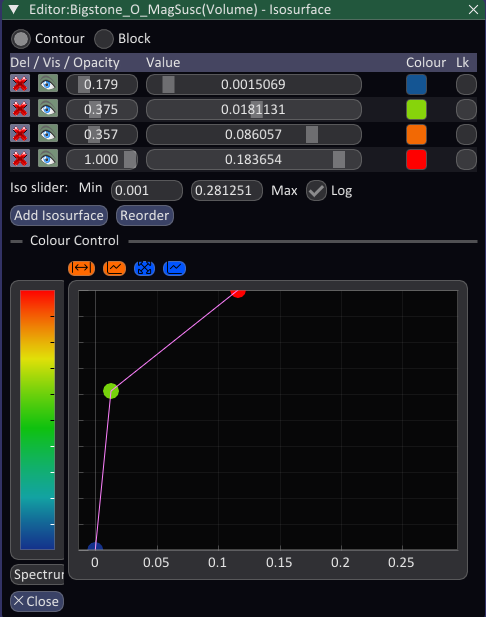
The isosurface table shows one row per isosurface, with the following controls per row:

Delete – Remove this isosurface.
Visible – Toggle display of this isosurface without removing it.
Opacity – Slider from 0 (transparent) to 1 (fully opaque).
Value – The isovalue slider. Drag to preview, release to compute the full surface.
Colour – The fill colour of the surface. By default this is driven by the colour scale (see Colour Control below); click to override it manually.
Lock – When ticked the colour is fixed to the manually chosen value and will not be updated by the colour scale.

Use Add Isosurface to append a new isosurface at the midpoint of the current slider range, and Reorder to sort them from lowest to highest isovalue (useful for correct transparency ordering).

The Iso slider min and max fields set the range of the isovalue slider for all isosurfaces. If the minimum value is greater than zero a Log checkbox appears to use a logarithmic slider scale, which is helpful when data spans several orders of magnitude.

The Colour Control section provides a colour scale that is applied to unlocked isosurfaces based on their isovalue.

Contours

Select Contour mode (the default) to render each isosurface as a classic single-value surface – exactly at the boundary where the attribute equals the specified isovalue. This is the best choice when you want to show a specific grade shell or structural boundary.

Blocks

Select Block mode to render each entry as a filled solid between a lower and an upper threshold value, showing all cells whose attribute falls within that range. This is equivalent to a threshold filter and is well suited to block model display, where you want to highlight all blocks above a certain cut-off grade.

Each entry has two value sliders – the lower and upper threshold – instead of a single isovalue. Enable Link threshold ranges to make the upper threshold of one entry automatically track the lower threshold of the next, so a set of colour-coded entries covers a continuous, gap-free range of values. Linking threshold ranges only really works if the isovalues have been reordered from lowest to highest.

Outline

The Outline visualisation draws the bounding box of the entire volume as a wireframe. This is useful as a lightweight reference to confirm that the volume is positioned and oriented correctly in the scene before computing more expensive visualisations. You cannot intersect an outline to get coordinates or centre the scene – it is decoration only.

Cell Edges

The Cell Edges visualisation draws the wireframe edges of every individual cell in the grid. This lets you inspect the cell geometry directly and is particularly useful for checking that mesh spacing and cell sizes are correct, or for displaying small block models where the block boundaries should be clearly visible. You can add this visualisation by right-clicking the layer and choosing Add Visualisation. Note that you cannot intersect an outline to get coordinates or centre the scene – it is decoration only.

For large grids this can generate a very large number of lines, so it is best used on coarser meshes or in combination with a clip object to limit the displayed region.