
Spatial Integration displays 2D seismic lines from SEGY files as curtains — vertical surfaces that follow the survey line through the scene and are coloured by trace amplitude. Curtains sit alongside your terrain, drillholes, volumes and GIS data, so a seismic line can be viewed in context and clipped, measured and interrogated like any other object.
SEGY support requires a Professional license.
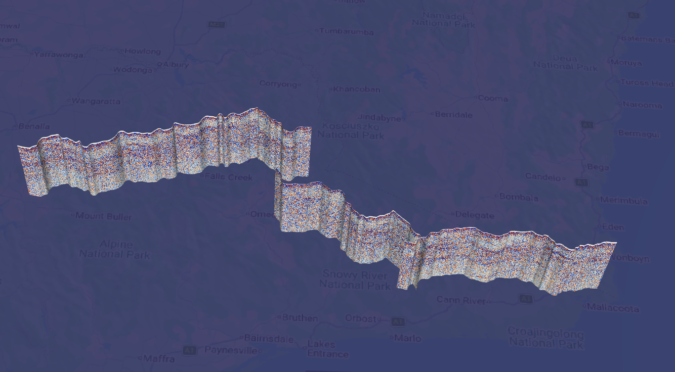
Two steps: import once, then load
A SEGY file is not read directly by the scene. It is first converted into a GeoTiff that carries the amplitudes and various other parameters encoded in the file. This conversion is done once per SEGY file; after that the GeoTiff loads in a moment and is what your project refers to.
Hover over the Surface icon in the left flyout and click Load SEGY…. You can also drag and drop .sgy, .segy or previously processed .tif files onto the scene or onto the Surface flyout button.
The Load SEGY dialog has two paths:
- Processed GeoTiff File — choose one or more GeoTiffs that Spatial Integration has already written and click OK. A curtain layer is created for each one.
- Import From SEGY… — opens the Import SEGY dialog described below, for SEGY files that have not been converted yet. When the conversion finishes, the curtain layers are created automatically, so you do not need to load the GeoTiffs by hand the first time.
Importing a SEGY file
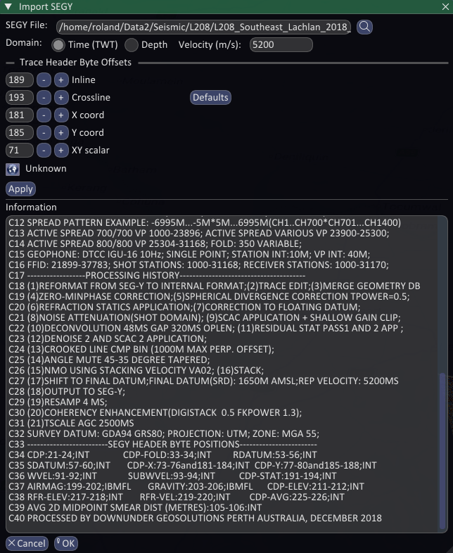
SEGY File — type a path or click the magnifier to browse. Several files can be selected at once, but they will all be imported using the same domain, velocity and byte offsets, so only batch files that come from the same processing run. A warning is shown while more than one file is selected.
Domain — whether the samples are in two way time or in depth. Spatial Integration detects this from the textual header (keywords such as TWT, TVD, DEPTH, and the units quoted against the sample interval), so it is normally already correct. Override it if the header is misleading.
Velocity (m/s) — only used for time sections. Samples are converted to elevation with a single constant velocity. Check the header text displayed in the import dialog for clues on what velocity to use if you’re not sure. The velocity is baked into the GeoTiff, so changing it means importing the SEGY again.
Trace header byte offsets
SEGY files vary in where they place their geometry, so the byte position of each field can be set:
- Inline and Crossline — line numbers, reported in the Information panel so you can confirm the file is being read sensibly.
- X coord and Y coord — the trace positions that place the curtain in the world.
- XY scalar — the field holding the coordinate scalar. A positive value multiplies the coordinates, a negative value divides by its magnitude.
Defaults restores the standard positions (189, 193, 181, 185 and 71). Your offsets are remembered between sessions, so a survey that uses non-standard positions only has to be set up once. Many processors list the byte positions they used in the textual header — the example above gives them on lines C33 to C39.
Coordinate reference system
Click the CRS button to set the coordinate system of the trace coordinates. Spatial Integration looks for one first in a .qpj file beside the SEGY, then for an EPSG code in the textual header, and shows "Unknown" if it finds neither. Setting the correct CRS matters — the curtain is transformed into the scene’s coordinate system when it is loaded. Note that seismic sections can also be displayed in Geographic coordinate systems if your area of interest spans a large area.
Apply and the Information panel
Apply reads the file’s metadata and scans the trace headers — the first, the last and around a thousand traces spread through the file — then fills the Information panel. It runs again automatically when you choose a file or press Defaults.
Read the panel before pressing OK. It reports the sample format, endianness, trace and sample counts, the sample interval, the detected domain, the coordinate scalar, the X and Y ranges, the line length and average trace spacing, the first and last trace positions, the inline and crossline ranges, and the complete textual header. Check that the line length and trace spacing are believable for the survey — that is the quickest test that the X, Y and scalar offsets are right.
Warnings appear in the same panel:
- Not a valid field position — the byte offset does not land on a real trace header field.
- First and last traces have the same coordinates — the X/Y offsets or the scalar are almost certainly wrong.
- X range extends beyond a single projection zone — a long line projected "out of zone". The coordinates are self consistent, but positions become progressively distorted away from the central meridian of the zone you select.
- File appears truncated — the data does not divide into whole traces. Re-copy the file from its source.
OK starts the conversion. If a GeoTiff already exists for a file you are asked before it is overwritten. Conversion runs in the background — the Load SEGY dialog shows a spinner and the number of imports remaining, and the log reports the trace count as it streams through the file and then the overview building. Large files take a while, but this only happens once.
The result is written next to the SEGY file with .tif appended, so L208.sgy produces L208.sgy.tif. It contains the amplitude and the elevation of every sample, the trace positions, the CRS and internal overviews. Keep it with your project; it is the file the project refers to from then on.
Elevation of the section
Time sections are hung from the seismic reference datum recorded in the trace headers, and the delay recording time of each trace is honoured, so a line that was shifted to a final datum during processing arrives at the right elevation. Depth sections use the sample interval and first sample depth, converted to metres using the units quoted in the textual header.
Remember that a time section is positioned with one constant velocity. It is correct enough to hang the line in the scene next to drilling and topography, but it is not an accurate depth conversion. If your two-way-time section does not match surface topography it may be due to single-velocity depth conversion.
Displaying a curtain
A curtain is a surface layer, so it appears in the Surface flyout with the usual visibility and opacity controls, and can be renamed, clipped and interrogated. It has no height or image sources — its geometry and its colours both come from the SEGY — so its Surface dialog only offers the Symbology tab.
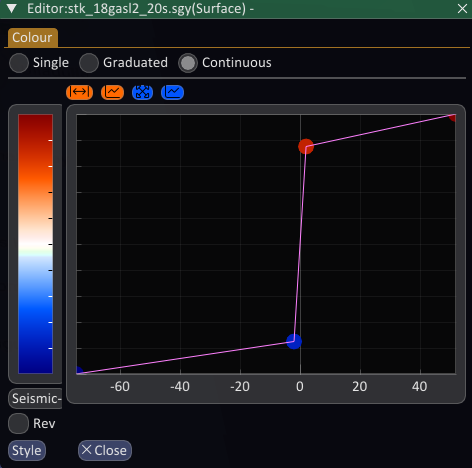
Curtains are coloured by Amplitude using a Continuous transform, initially a reversed greyscale ramp scaled to the amplitude range of the file. Click the label under the colour bar to choose a different ramp — "Seismic" gives the familiar blue and red — and tick Rev if you want to reverse it.
Seismic amplitudes are strongly peaked around zero, so almost all the useful contrast lives in a narrow band in the middle of the range. Drag the anchor points close to zero apart or together to change the gain, double click on the transform to add an anchor point, and right click on one to delete it. The steep central step in the picture above is what produces a well balanced section.
If something looks wrong
- The line plots as a point, or the trace spacing is absurd — the X and Y byte offsets or the XY scalar are wrong. Fix them, press Apply, and check the line length in the Information panel.
- The section is in the wrong place — the CRS of the trace coordinates is wrong or missing.
- The section is at the wrong depth or too tall — check the domain and, for time sections, the velocity.
- "Unsupported SEGY sample format (3 byte integer)" — the 3 byte integer formats cannot be converted. Ask for the data in another format.
- The GeoTiff will not load — only GeoTiffs written by Spatial Integration’s SEGY import can be opened as curtains. An ordinary GeoTiff is reported as invalid.